Melikerion guide

The system accepts exactly two files: one that contains processing instructions (configuration file) and another that contains the tabulated data with column headings (data file). The instructions can be of three main types: NameVariable defines the column (heading) in the data file that lists the sample labels, which need not be numbers. InputVariable defines a column of training data for the SOM. Note that you should list multiple input variables in the configuration file. TestVariable indicates data that is not to be used in the training of the model, but can be used for statistical significance estimates. ResponseVariable can be used to guide the SOM in a semi-supervised manner (automatic scaling of inputs). An artificial dataset is available for testing on the submission page.

You can set the map size also manually with the MapSize instruction. See the example configuration file for details.

The default input file format is tabulator separated text. If you are using spreadsheet software to prepare your files (e.g. MS Excel), please make sure that you save/export the data into a text file before submitting. For security reasons, non-alphanumeric characters may be converted to numeric codes during processing; it is thus best to use only the basic English alphabet to avoid confusion.

Prototypes

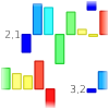From a practical point of view, the self-organizing map is nothing more than a collection of multi-variate profiles of the input variables. The output file proto.svg contains a visualization of these profiles. The bar plots describe the relative level of each input on a given map unit and the numbers next to the bars indicate the coordinate on the map. For large SOMs, only a limited set of all profiles is depicted to prevent excessive image files; the systems adds a notification “reduced prototype visualization” if this is the case. The file protolegend.svg links the variables to the bar colors, so that the figure can be correctly interpreted. If you are using response variables, the input scales are listed in protoscales.txt.

Map colorings (component planes)

The collection of prototypes can also be viewed one variable at the time. The map units can be colored according to the level of a given variable, which need not be an input. This is analogous to a geographic map that is painted according to the age of inhabitants in administrative districts, for instance. Put differently, only the positions of the data samples (e.g. patients) on the map is used, and the level of the variable under interest is determined as an average of those samples that reside on any given map unit.

The result files ending with _plane.svg contain the map colorings for every variable included in the analyses (inputs or outputs). The same information is also available in numerical format (arranged into a matrix) in the files ending with _plane.txt. Not all the maps are colored with the same intesity of red or blue; this is due to the statistical normalization procedure that is discussed next.

Statistical significance and confidence intervals

Comparing the colorings of variables with missing data, different types of distributions and value ranges may make the overall intepretation of the results challenging. Furthermore, there is no straightforward statistical test to verify the significance of the observed prototypes and spatial patterns.

Here the above problems have been solved by numerical approximations: the P-values of non-input variables are estimated by permutation analysis, and the model variance (basis of confidence intervals) is estimated by a bootstrapping algorithm. This requires some computational resources, but for modern hardware the processing time is minutes rather than hours, which is very efficient considering the efforts in data collection in medical sciences, for example.

Files ending with _null.svg contain the empirical null distribution for the hypothesis that the variable under interest is not in any way related to the layout of the data samples on the map. The histogram describes the values of the test statistic (a measure of regional variation) from the permutation rounds. The null distribution has an approximately Gaussian shape, and the P-value is computed according to the standard normal density function. Note that P-values cannot be computed for the input variables since they are directly responsible for the layout. The same procedure is nevertheless repeated for every variable to make the color scales comparable. A summary of the results is tabulated in pvalues.txt.

Confidence intervals (95%) for each coloring are stored in files ending with _c0025.txt (2.5 percentile) and _c0975.txt (97.5 percentile). The percentiles are obtained by bootstrapping: random sample sets (with replacement) are drawn repeatedly and the coloring is recomputed at each iteration. For input variables this may give optimistic results, since a full simulation of model variance would involve recomputing the SOM at each iteration. Note also that due to the lack of constraits for the SOM shapes the full approach would not be accurate either in general.

Map structure and quality

Besides statistical considerations, the map quality is also determined by its capacity to describe the salient aspects of the dataset. A key property of any unsupervised learning method is to detect the presence of clusters. For the SOM, distinct groups (if present) will be reflected by differences in adjacent prototypes when moving across the map. This so called U-matrix is often depicted as distances between map units, but in many cases this makes it difficult to relate the U-matrix to the map colorings. Here the focus is on the rate of change rather than unit distances; hence the “U-book” transforms into just another coloring of the map in the result files ubook.svg and ubook.txt.

The SOM training algorithm is iterative and as such subject to incomplete model fitting. Two complementary error measures can be utilized to investigate the map structure. First, the average vector difference between samples and their best matching map units indicates how well the model can explain the variations in the data (quantization error). Another approach is to look at the best and second best matching units: if they are adjacent, the samples localize to a small area on the map, which is a sign of descriptive efficiency (low topographic error). During the training process, both measures usually decline until the topographic error begins to grow if the map smoothing function is inadequate.

One or two numbers is insufficient to illustrate the map structure so the two measures are estimated locally on each map unit. This way areas of poor fit and the samples therein can be identified and their impact considered when interperting the results. The quantization error coloring is stored in qbook.svg and qbook.txt, and the topographic coloring in tbook.svg and tbook.txt.

Sample positions, outliers and missing data

A few unusual samples can have a significant impact on the shape of the SOM and it is therefore important to carefully investigate those parts of the map where errors are high. On the other hand, one can also look at the data and determine those samples that do not fit the model. The histogram of the sample quantization errors is depicted in qerrors.svg and the error magnitudes are listed in qerrors.txt. Data items with unusually large errors may be erroneous and need to be removed or at least checked in detail.

Sometimes it may be interesting to study the map locations of inidividual samples, especially if they represent time series data and the trajectories on the map contain important dynamic features. The sample positions are thus stored in bmus.txt for subsequent analyses.

The SOM produces estimates for missing values in the training set, so it can be used for data imputation. Similarly, the test and response variables can be estimated from the map structure. The imputed training set (with missing values replaced by estimates) is stored in imputed_inputs.txt and the estimated output data are stored in estimated_testvars.txt and estimated_responses.txt.